CryoET Background

This page summarises the conceptual and mathematical background behind SUSAN: phase-contrast imaging and the Contrast Transfer Function, the missing wedge, Subtomogram Averaging (classical and high-resolution), and the substack formulation that SUSAN is built on.

Phase contrast and the Contrast Transfer Function

Biological specimens scatter electrons only weakly, so the electron microscope introduces a controlled amount of defocus to convert phase modulations of the electron wave into measurable intensity contrast (phase-contrast imaging). The result is that each recorded projection is not a clean projection of the specimen’s electrostatic potential but is modulated by the Contrast Transfer Function (CTF):

\[\text{CTF}(s) = -\sin\!\Bigl( \tfrac{\pi}{2} C_s \lambda^3 s^4 + \pi \lambda \Delta_z s^2 + \phi_{A_c} \Bigr),\]

where \(s\) is the spatial frequency, \(C_s\) is the spherical aberration coefficient, \(\lambda\) is the electron wavelength, \(\Delta_z\) is the defocus, and \(\phi_{A_c}\) accounts for amplitude contrast. The CTF oscillates with frequency, creating phase reversals and zero crossings that suppress or invert specific Fourier components. Accurate modelling and correction of the CTF is therefore essential for achieving high-resolution reconstructions.

In CryoET, defocus varies across the field of view and changes with specimen depth, so the CTF must be estimated and ideally corrected on a per-projection, per-particle basis.

The missing wedge

Mechanical constraints limit the tilt range of the specimen stage (typically \(\pm 60°\)). The resulting missing wedge is a cone-shaped region in Fourier space that is never sampled, regardless of how many projections are collected. The missing wedge causes characteristic elongation artefacts in tomogram reconstructions and introduces anisotropic resolution. Subtomogram averaging compensates for the missing wedge by combining particles in many different orientations, so that different copies fill in the missing Fourier information from one another.

Subtomogram Averaging

Let \(V^*\) denote the unknown structure of the target protein, \(\mathbf{P} = \{P_j\}_{j=1}^{N_\text{proj}}\) the acquired tilt series, \(\boldsymbol{\mathcal{T}}^\text{tilt} = \{\mathcal{T}^\text{tilt}_j\}_{j=1}^{N_\text{proj}}\) the corresponding tilt geometry, and \(\boldsymbol{\mathcal{C}} = \{C_j\}\) the CTF parameters estimated from \(\mathbf{P}\). The tomogram \(T\) is reconstructed from \(\mathbf{P}\) using \(\boldsymbol{\mathcal{T}}^\text{tilt}\) and \(\boldsymbol{\mathcal{C}}\). Each particle \(i\) contributes a subtomogram \(Y_i\), cropped from \(T\), which contains a rotated and translated copy of \(V^*\):

\[Y_i = \mathcal{T}^v_i\, V^*,\]

where \(\mathcal{T}^v_i\) is the unknown spatial transformation (rotation and translation) for particle \(i\), and \(\boldsymbol{\mathcal{T}}^v = \{\mathcal{T}^v_i\}_{i=1}^{N_\text{par}}\) their collection. The goal of StA is to estimate \(V \approx V^*\) from the set \(\mathbf{Y} = \{Y_i\}_{i=1}^{N_\text{par}}\). Averaging \(N_\text{par}\) aligned copies improves the signal-to-noise ratio proportionally to \(\sqrt{N_\text{par}}\), enabling high-resolution reconstruction even from inherently noisy CryoET data. Throughout this section, capital letters denote Fourier-space quantities and boldface denotes collections.

Classical StA

Given the subtomograms \(\mathbf{Y}\) and their unknown orientations \(\boldsymbol{\mathcal{T}}^v\), classical StA solves the least-squares problem

\[V = \arg\min_{\boldsymbol{\mathcal{T}}^v,\, V} \bigl\| \mathbf{Y} - \boldsymbol{\mathcal{T}}^v V \bigr\|_2^2\]

by alternating between (i) an orientation search via exhaustive 3D cross-correlation and (ii) computing the aligned average. The missing wedge is accounted for in both steps: during the orientation search, unsampled Fourier voxels are masked to avoid correlating against missing data; during averaging, the same mask prevents missing-wedge artefacts from propagating into the consensus volume. Because the quality of \(\mathbf{Y}\) depends directly on the accuracy of \(\boldsymbol{\mathcal{C}}\) and \(\boldsymbol{\mathcal{T}}^\text{tilt}\) used to reconstruct \(T\), classical StA is fundamentally limited by the initial estimates of these imaging parameters.

High-resolution StA

High-resolution StA addresses this limitation through an iterative refinement loop. Using the current high-SNR average \(V\) as a reference, it refines \(\boldsymbol{\mathcal{T}}^\text{tilt}\) per projection by projection-matching against \(\mathbf{P}\); each per-projection update is regularised to prevent noise-driven drift of the geometric parameters. \(\boldsymbol{\mathcal{C}}\) is refined analogously. The improved parameters are then used to reconstruct an updated \(T\) and subtomograms \(\mathbf{Y}\), and classical StA yields a higher-resolution estimate of \(V\). Each cycle reveals finer structural detail, because every iteration improves the imaging parameters that determine the quality of \(\mathbf{Y}\).

Resolution assessment

Resolution is assessed with the Fourier Shell Correlation (FSC) between two independently processed half-datasets; the reported resolution is the spatial frequency at which FSC falls below the 0.143 threshold. For two half-maps \(V_a\) and \(V_b\), the FSC at shell \(S(s)\) is:

\[FSC(s) = \frac{ \displaystyle\sum_{\mathbf{k} \in S(s)} V_a(\mathbf{k})\,\overline{V_b(\mathbf{k})} }{\sqrt{ \displaystyle\sum_{\mathbf{k} \in S(s)} |V_a(\mathbf{k})|^2 \cdot \displaystyle\sum_{\mathbf{k} \in S(s)} |V_b(\mathbf{k})|^2 }}\]

A useful property of the FSC is its invariance to isotropic spectral envelopes. If both half-maps are modulated by the same radially symmetric factor \(E(s)\), the \(|E(s)|^2\) terms cancel between numerator and denominator, leaving \(FSC(s)\) unchanged. This makes the FSC a reliable resolution estimator even when signal amplitudes are attenuated by the CTF, radiation damage, or other frequency-dependent effects.

SUSAN: Substack Analysis

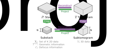
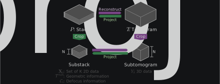
SUSAN reformulates the StA problem by replacing the subtomogram \(Y_i\) with its corresponding substack \(\mathbf{X}_i\) as the fundamental data unit. All processing, including alignment, CTF correction, and averaging, operates directly on \(\mathbf{X}_i\), extracted on-the-fly from the original tilt series \(\mathbf{P}\). Tomograms serve only for initial particle picking and visual validation; no tomogram reconstruction is needed inside the iterative refinement loop.

Projected cross-correlation

The substack \(\mathbf{X}_i = \{X_{i,j}\}_{j=1}^{N_\text{proj}}\) collects the 2D projections of particle \(i\), extracted from \(\mathbf{P}\) using the tilt geometry \(\boldsymbol{\mathcal{T}}^\text{tilt}\) and CTF parameters \(\boldsymbol{\mathcal{C}}_i\):

\[\mathbf{X}_i = \boldsymbol{\mathcal{C}}_i\operatorname{Proj}_{\boldsymbol{\mathcal{T}}^\text{tilt}}(Y_i).\]

Because the reconstruction operator is linear, \(Y_i\) can be recovered from \(\mathbf{X}_i\) by weighted backprojection after CTF correction. Substituting this expression into the Fourier-space cross-correlation and using linearity yields the projected cross-correlation (pCC), where \(\Phi_{nD}\) denotes the \(n\)-dimensional cross-correlation operator:

\[\Phi_{3D}(Y_i,\, V) = \Phi_{3D}(\operatorname{Rec}_{\boldsymbol{\mathcal{T}}^\text{tilt},\boldsymbol{\mathcal{C}}_i}\!(\mathbf{X}_i),\, V) = \operatorname{Rec}_{\boldsymbol{\mathcal{T}}^\text{tilt}}\! \bigl( \Phi_{2D} \bigl( \mathbf{X}_i,\; \boldsymbol{\mathcal{C}}_i\operatorname{Proj}_{\boldsymbol{\mathcal{T}}^\text{tilt}}(V) \bigr) \bigr).\]

The 3D cross-correlation is therefore the reconstruction of the per-projection 2D cross-correlations between each substack projection \(X_{i,j}\) and the corresponding forward projection of the reference, computed exactly with no approximation to the alignment metric. All per-particle computation is in 2D; the only 3D step is a small localised reconstruction of the CC peak region, reducing complexity from \(\mathcal{O}(N^3 \log N)\) to \(\mathcal{O}(N_\text{proj} N^2 \log N + L^3)\), where \(L \ll N\) is the half-search radius.

The pCC formulation has the following consequences:

• Missing wedge in the CC domain. The missing wedge is no longer present in the data being correlated; it manifests instead as artefacts in the reconstructed CC volume. Because alignment uses only the peak location and its relative magnitude, these artefacts do not affect alignment accuracy.

• Near-zero 3D computation per particle. All heavy computation runs in 2D on the GPU; the single 3D operation per particle (the localised CC reconstruction) covers only a small volume of side \(2L\).

• Per-projection CTF correction. Because \(\mathbf{X}_i\) is extracted from the raw tilt series, the per-projection CTF parameters \(C_j\) are applied and refined in 2D, which is the natural and exact domain for these corrections.

• No subtomogram storage. Substacks are extracted on-the-fly into GPU memory; no subtomogram or tomogram is written to disk inside the refinement loop.

• Additive overlap contribution. Cross-correlation is a linear operator, so the contribution of any overlapping neighbouring particle is additive and separable: \(\Phi(Y_\text{target} + Y_\text{neighbour},\, V) = \Phi(Y_\text{target},\, V) + \Phi(Y_\text{neighbour},\, V)\). Across a dataset where neighbouring particles adopt many different orientations, the neighbour term is diffuse in the CC volume and does not bias the peak used for alignment.

Cumulative Fourier Shell Correlation

The raw pCC metric is sensitive to spectral coloring from CTF modulation, radiation damage, and high-frequency noise. SUSAN replaces the raw cross-correlation with a shell-wise spectral normalisation inspired by the FSC, yielding the cumulative Fourier Shell Correlation (cFSC).

Define the shell-normalised counterpart \(\tilde{A}\) of a volume \(A\) by dividing each Fourier coefficient \(A(\mathbf{k})\) by the root sum of squares of its shell:

\[\tilde{A}(\mathbf{k}) = \frac{A(\mathbf{k})}{\|A\|_{S(s)}}, \qquad \|A\|_{S(s)} = \sqrt{\sum_{\mathbf{k}' \in S(s)} |A(\mathbf{k}')|^2}.\]

Summing the per-shell FSC across all shells then gives:

\[\operatorname{cFSC}(Y_i,\, V) = \sum_s \operatorname{FSC}_{Y_i,V}(s) = \Phi_{3D}\!\left(\tilde{Y}_i,\; \tilde{V}\right).\]

The cFSC is therefore a standard 3D cross-correlation applied to the shell-normalised volumes. This normalisation gives it three key properties:

• Envelope invariance. Any isotropic spectral envelope (CTF, B-factor decay, radiation damage) applied to either volume is constant within each shell and cancels in the shell-wise denominator. The cFSC similarity score is therefore unaffected by spectral coloring, for the same reason the FSC is invariant to envelopes when measuring resolution.

• Shift invariance. A spatial shift of the reference introduces per-coefficient phase factors of unit magnitude, which do not change the shell energy. The peak height is preserved under shifts, and the peak location continues to encode the relative displacement.

• SNR weighting. Shells with low signal energy contribute little to the total score without requiring an explicit noise-power estimate. Unlike radial whitening, which forces a flat spectrum and can amplify noise in high-frequency shells, the cFSC preserves the natural relative contribution of each shell.

For computational efficiency, the cFSC is computed per projection as a cumulative Fourier Ring Correlation (cFRC): each 2D projection of the substack is normalised shell-wise, correlated with the corresponding normalised reference projection, and the 2D results are backprojected to reconstruct the 3D similarity volume. The additional cost relative to raw pCC is negligible.

SUSAN optimization objective

The complete SUSAN problem is a joint optimization over the reference, particle orientations, tilt geometry, and CTF:

\[V,\, \boldsymbol{\mathcal{T}}^v,\, \boldsymbol{\mathcal{T}}^\text{tilt},\, \boldsymbol{\mathcal{C}} \;=\; \underset{V,\, \boldsymbol{\mathcal{T}}^v,\, \boldsymbol{\mathcal{T}}^\text{tilt},\, \boldsymbol{\mathcal{C}}} {\arg\max}\; \operatorname{cFSC}\!\bigl( \mathbf{X},\; \boldsymbol{\mathcal{C}}\,\boldsymbol{\mathcal{T}}^\text{tilt}\,\boldsymbol{\mathcal{T}}^v V \bigr),\]

where \(\mathbf{X} = \{\mathbf{X}_i\}\) collects all substacks. This is solved by alternating among three sub-problems:

• Particle orientations \(\boldsymbol{\mathcal{T}}^v\): with \(V\), \(\boldsymbol{\mathcal{T}}^\text{tilt}\), and \(\boldsymbol{\mathcal{C}}\) fixed, pCC reconstructs the 3D cross-correlation from per-projection 2D correlations for each candidate orientation. Finding the orientation that maximises it is the direct projection-domain equivalent of classical StA.

• Tilt geometry and CTF \(\boldsymbol{\mathcal{T}}^\text{tilt}\), \(\boldsymbol{\mathcal{C}}\): with \(V\) and \(\boldsymbol{\mathcal{T}}^v\) fixed, each per-projection parameter is refined by maximising the 2D cross-correlation between the substack projection and the corresponding forward projection of the reference. No 3D reconstruction is required for this step; this is the high-resolution component of the pipeline.

• Reference \(V\): with all parameters fixed, the reference is updated by direct Fourier reconstruction with Wiener inversion: substack projections are accumulated into 3D Fourier-space numerator and denominator volumes, weighted by the per-projection CTF, and divided to yield the CTF-deconvolved reference.

Angular conventions

Both orientation sub-problems are searched with the same cone/in-plane sampling and both store their result as a ZYZ Euler triplet, built as

\[R(\theta_0,\theta_1,\theta_2) = R_z(\theta_0)\,R_y(\theta_1)\,R_z(\theta_2).\]

The two triplets do not read the same way, because the two rotations sit at opposite ends of the projection chain. Writing the full reference-to-image transform for particle \(i\) and projection \(j\),

\[\underbrace{R^\text{prj}_{ij}}_{\texttt{prj\_eu}}\; \underbrace{R^\text{tilt}_{j}}_{\texttt{.tomostxt}}\; \underbrace{R^\text{ali}_{i}}_{\texttt{ali\_eu}},\]

ali_eu is the innermost factor and prj_eu the outermost one. Each search perturbs its own rotation in the frame that matters for it — the reference frame for the 3D search, the projection frame for the 2D one — so the increment is composed on the right of ali_eu and on the left of prj_eu. That single difference mirrors the meaning of the three stored angles:

	ali_eu (3D alignment)	prj_eu (2D refinement)
maps	reference → tomogram	tilt geometry → image
increment	right-multiplied	left-multiplied
cone axis	particle Z in the tomogram	viewing direction
\(\theta_0\)	cone azimuth	in-plane rotation
\(\theta_1\)	cone polar	cone polar
\(\theta_2\)	in-plane rotation	cone azimuth, as \(180^\circ-\theta_2\)

So for ali_eu the triplet reads (azimuth, polar, in-plane) and a pure in-plane search moves \(\theta_2\) alone, whereas for prj_eu it reads (in-plane, polar, azimuth) and a pure in-plane search moves \(\theta_0\) alone. The polar angle is \(\theta_1\) in both.

The sampling parameters are unaffected by this and keep their literal meaning in both searches: cone_range is the full aperture of a cone centred on the current axis — the particle’s own Z for 3D, the viewing direction for 2D — so a sample at polar \(\theta\) displaces that axis by exactly \(\theta\) for every azimuth, and inplane_range spans a rotation about that same axis that leaves it fixed. Only the slot the result is stored in differs.

Note

The ZYZ parametrisation is degenerate at \(\theta_1 = 0\), where \(R = R_z(\theta_0 + \theta_2)\) and only the sum is determined. The stored \(\theta_0\) and \(\theta_2\) are then individually ill-conditioned — a particle whose axis nearly coincides with the cone axis can show both angles swinging by degrees between iterations while the rotation itself barely moves. Use the rotation matrix, or \(\theta_0 + \theta_2\), for per-particle statistics and convergence diagnostics in that regime; never the two angles separately.

Spectral weighting in the reconstruction

The Wiener inversion of the previous section accumulates two Fourier volumes over every contributing projection \(j\) and divides them:

\[V(\mathbf{k}) \;=\; \frac{\sum_j\, w_j(s)\, C_j(s)\, X_j(\mathbf{k})} {\sum_j\, \bigl[\, C_j(s)^2 \;+\; 1/\mathrm{SSNR}(s) \,\bigr]}, \qquad s = |\mathbf{k}| / (N \cdot \mathrm{apix}),\]

where \(s\) is the spatial frequency in 1/Å. Three separate envelopes enter this expression, and they are not interchangeable: what distinguishes them is not their shape, which is identical, but whether they appear in the denominator.

CTF and B-factor (def_Bfct) form the transfer term \(C_j(s) = \mathrm{CTF}_j(s)\cdot e^{-s^2 B_j/4}\). Because \(C_j\) appears once in the numerator and squared in the denominator, the B-factor is compensated: the division removes it, and the reconstruction attempts to deconvolve it. It describes an envelope that the reconstruction should undo.

Exposure filter (def_ExFl) forms the weight \(w_j(s) = \mathrm{BP}(s)\cdot e^{-s^2 D_j/4}\), together with the bandpass. It appears in the numerator only. It is therefore uncompensated: it survives into the final map and permanently attenuates projection \(j\), and, because the denominator still receives that projection’s full \(C_j^2\), a heavily filtered projection also dilutes the contribution of the others in that shell. It describes an envelope that the reconstruction should keep.

Both are stored in Ų and use the same functional form, \(e^{-s^2 X/4}\). The choice of field is therefore a choice of semantics:

Field	Behaviour	Use it for
def_Bfct	Compensated	An envelope you want deconvolved. Part of the CTF model.
def_ExFl	Uncompensated	An envelope you want to persist in the map, e.g. dose weighting.

Ad-hoc SSNR (susan.utils.datatypes.ssnr) contributes the regulariser \(1/\mathrm{SSNR}(s)\), with \(\mathrm{SSNR}(s) = 10^{3S} e^{-100 F s}\). Note that it is added once per projection, so for a voxel reached by \(n\) projections the denominator is \(n\bigl(\langle C^2\rangle + 1/\mathrm{SSNR}\bigr)\) and \(n\) cancels. Two consequences follow:

• \(S\) and \(F\) parameterise the SSNR of a single projection, not of the reconstructed map. They must not be read off a half-map FSC directly: the map SSNR exceeds the per-projection SSNR by the Fourier-space redundancy \(n(s)\).

• The resulting filter is invariant to the number of particles and tilts. Adding particles does not change the shape of the roll-off.

The effective radial filter applied to the map is \(H(s) = \langle C^2\rangle / \bigl(\langle C^2\rangle + 1/\mathrm{SSNR}(s)\bigr)\), which reaches half power near \(100 F / (6.91 S - 0.69)\) Å. With the usual \(S = 1\), this is approximately \(16 F\) Å, so \(F\) behaves as a resolution knob: \(F \approx d/16\) keeps the Wiener inversion transparent out to \(d\) Å.

Note

The exposure filter is applied only by the 'wiener', 'pre_wiener' and 'wiener_ssnr' reconstruction policies. 'none' and 'phase_flip' ignore def_ExFl entirely.